Where is everybody?
— Enrico Fermi
The omnipresence of uncertainty is part of why making predictions and decisions is so hard. We at Lumina advocate treating uncertainty explicitly in our models using probability distributions. Sadly this is not yet as common as it should be. A recent paper “Dissolving the Fermi Paradox” (2018) is a powerful illustration of how including uncertainty can transform conclusions on the fascinating question of whether our Earth is the only place in the Universe harboring intelligent life. The authors, Anders Sandberg, Eric Drexler and Toby Ord (whom we shall refer to as SDO), show elegantly that the apparent paradox is simply the result of the mistake of ignoring uncertainty, what Sam L. Savage calls the Flaw of Averages. In this article, we review their article and embed a live Analytica version of their model that you can explore.
The Fermi Paradox
One day in 1950, Enrico Fermi, the Nobel prize-winning builder of the first nuclear reactor, was having lunch with a few friends in Los Alamos. They were looking at a New Yorker cartoon of cheerful aliens emerging from a flying saucer. Fermi famously asked “Where is everybody?”. Given the vast number of stars in the Milky Way Galaxy and the likely development of life and extraterrestrial intelligence, how come no ETs have come to visit or at least been detected? This question came to be called the “Fermi Paradox”. Ever since, it has bothered those interested in the existence of extraterrestrial intelligence and whether we are alone in the Universe.
The Flaw of Averages on steroids

Sam L. Savage, in his book, The Flaw of Averages, shows how ignoring uncertainty and just working with a single mean or “most likely” value for each uncertain quantity can lead to misleading results. To illustrate how dramatically this approach can distort your conclusions, SDO offer a toy example. Suppose there are nine factors that multiplied together give the probability of extraterrestrial intelligence (ETI) arising on any given star. If you use a point estimate of 0.1 for each factors, you could infer that there is a 10^{-9}10−9 probability of any given star harboring ETI. There are about 10^{11}1011 stars in the Milky Way, so the probability that no star other than our own has a planet harboring intelligent life would be extremely small, (1-10^{-9})^{100B} ≈ 3.7\times 10^{-44}(1−10−9)100B≈3.7×10−44. On the other hand, suppose that, based on what we know, each factor could be anywhere between 0 and 0.2, and assign a uniform uncertainty over this interval, using the probability distribution, Uniform(0, 0.2). If you combine these distributions probabilistically, using Monte Carlo simulation for example, the mean of the result is 0.21–over 5,000,000,000,000,000,000,000,000,000,000,000,000,000,000 times more likely!
The Drake equation
Frank Drake, a radio astronomer who worked on the search for extraterrestrial intelligence (SETI), tried to formalize Fermi’s estimate of the number of ETIs. He suggested that we can estimate N, the number of detectable, intelligent civilizations in the Milky Way galaxy from what is now called the “Drake equation”. It is sometimes referred to as the “second most-famous equation in science (after E= mc2)”:

N= R^* \times f_p \times n_e \times f_l \times f_i \times f_c \times LN=R∗×fp×ne×fl×fi×fc×L
Where
R^*R∗ is the average rate of formation of stars in our galaxy,
f_pfp is the fraction of stars with planets.
n_ene is the average number of those planets that could potentially support life.
f_lfl is the fraction of those on which life had actually developed;
f_ifi is the fraction of those with life that is intelligent; and
f_cfc is the fraction of those that have produced a technology detectable to us.
LL is the average lifetime of such civilizations
Many have tried to refine this calculation since Drake first proposed it in 1961. Most have estimated a large number for N, the number of detectable extraterrestrial civilizations. The contradiction between expected proliferation of detectable ETs and their apparent absence is what came to be called the “Fermi paradox” after the famous lunch conversation.
Past explanations of the Fermi Paradox
 Many have tried to resolve the apparent paradox: Maybe advanced civilizations avoid wasteful emission of electromagnetic radiation into space that we could detect. Maybe interstellar travel is simply impossible. Or if it is technically possible, all ETs have decided it’s not worth the effort. Or perhaps ETs do visit us but choose to be discreet, deeming us not ready for the shock of contact. Maybe there is a Great Filter that makes the progression of life to advanced stages exceedingly rare. Or perhaps, the development of life from lifeless chemicals (abiogenesis) and/or the evolution of technological intelligence are just so unlikely that we are in fact the only ones in the Galaxy. Or, even more depressingly, perhaps those intelligent civilizations that do emerge all manage to destroy themselves in short order before perfecting interstellar communication—as indeed we Earthlings may plausibly do ourselves.
Quantifying uncertainty in the Drake equation
SDO propose a nice way to resolve the apparent paradox without resorting to any speculative explanation. Recognizing that most of the factors of the Drake equation are highly uncertain, they express each factor as a probability distribution that characterizes the uncertainty based on their review of the relevant scientific literature. They then use simple Monte Carlo simulation to estimate the probability distribution on N, and hence the probability that N<1N<1 — i.e. that there are zero ETIs to detect. They estimate this probability at about 52% (our reimplementation of their model comes up with 48%). In other words, we shouldn’t be surprised at our failure to observe any ETI because there is a decent probability that there aren’t any. Thus, we may view the Fermi paradox as due simply to Sam Savage’s “Flaw of Averages”: If you use only “best estimates” and ignore the range of uncertainty in each assumption, you’ll end up with a misleading result.
For most factors. the uncertainty ranges over many orders of magnitude. For all except one factor, SDO represent its uncertainty using a Log-Uniform distribution, assuming that each order of magnitude is equally likely over its range. In other words, the logarithm of the value is uniformly-distributed. This table summarizes their estimated uncertainty for each factor.
| Factor | Distribution | Description | |
|---|---|---|---|
| R^*R∗ | LogUniform(1, 100) |
Rate of star formation (stars/year) | |
| f_pfp | LogUniform(0.1, 1) |
Fraction of stars with planets | |
| n_ene | LogUniform(0.1, 1) |
Number of habitable planetary objects per system with planets (planets/star) | |
| f_lfl | Version 1: LogNormal”1-e^{-e^{m}}1−e−em where m~ Normal(0,50) |
Version 2:“t V \lambdatVλ version”1-e^{-t V \lambda}1−e−tVλt\simt∼ LogUniform(1e7, 1e10)V\simV∼ LogUniform(1e2, 1e15)\lambda\simλ∼ LogUniform(1e-188, 1e15) |
Fraction of habitable planets that develop life. Abiogenesis refers to the formation of life out of inanimate substances.t\simt∼ Time avail. for abiogenesis (years)V\simV∼ Volume of substrate for abiogenesis (m^3m3)\lambda\simλ∼ Rate of abiogenesis (events per m^3m3 years)The scientific notation 1e15 is a way of writing 10^{15}1015, and so on. |
| f_ifi | LogUniform(0.001, 1) |
Fraction of planets with life that develops intelligence | |
| f_cfc | LogUniform(0.01, 1) |
Fraction of intelligent civilizations that are detectable | |
| LL | LogUniform(100, 1e10) |
Duration of detectability (years) |
SDO present two ways to estimate f_lfl, the fraction of habitable planets that develop life. Both use the form 1 – e^{-r}1−e−r as the probability that one or more abiogenesis events occur, assuming a Poisson-process with rate rr. In Version 1 they estimate a Lognormal distribution directly for rr. Version 2 decomposes rr into a product of three other quantities, t V \lambdatVλ , and assigns a loguniform to each one. (It is not clear to us that these three subquantities are any easier to estimate!) At the risk of stating the obvious, the ranges for f_lfl used by SDO are enormous in either version.
We couldn’t tell from the text of the paper alone which results used which version, so we included both versions in our model. This table gives some results from these models.
| N = # detectable planets in Milky Way | Pr(N<1) “we are alone” |
Pr(N>100M) “Teeming with intelligent civilizations” |
||
|---|---|---|---|---|
| Median | Mean | |||
| Reported in SDO | 0.32 | 27 million | 52% | – |
| Version 1 with uncertainty | 1.8 | 27.8 million | 48% | 1.9% |
| Version 2 with uncertainty | 9.9e-67 | 8.9M | 84% | 0.6% |
| Version 1 with point estimates | 2000 | 0% | 0% | |
| Version 2 with point estimates | 1e-66 | 100% | 0% | |
| f_l = 16%fl=16 | 500 | 8.9 million | 17% | 1.2% |
| f_l\simfl∼ Beta(1, 10) | 170 | 5 million | 23% | 1.4% |
The top row, “Reported in SDO”, shows the numbers from their text. The rest are from our Analytica implementation of their model. Their reported values seem more consistent with Version 1; but other results in their paper seem more consistent Version 2. We believe our implementation of both versions reflects those described in the paper. We even examined their Python code in a futile attempt to explain why our results aren’t an exact match. We have emailed the first author in the hope he can clarify the situation. While we can’t reproduce their exact results the discrepancies do not affect their broad qualitative conclusions.
The rows, Versions 1 and 2 with uncertainty, use SDO’s full distributions. The rows, Versions 1 and 2 with point estimates, use the median of their distributions as a point estimate for each of the seven factors of the Drake Equation or 9 parameters for Version 2. In Version 1 with uncertainty, the mean for N is four orders of magnitude larger than the corresponding point estimate. In Version 2 with uncertainty, it is 73 orders of magnitude larger than the corresponding point estimate.
The P(N<1) column shows the probability that there is no other detectable civilization in the Milky Way. The fact that it is so high means that we should not be surprised by Fermi’s observation that we haven’t detected any extraterrestrial civilization. In each case with uncertainty, there is a substantial probability (from 17% to 84%) that no other detectable civilization exists. We added a last column with the probability that our galaxy is absolutely teeming with life— with over 100 million civilizations, or 1 out of every thousand stars having a detectable intelligent civilization. The uncertain models give us between 0.6% and 1.9% of this case.
Explore the model yourself
Our Analytica model is running here where you can explore. (or, click here to run it in its own browser tab).
https://acp.analytica.com/view?invite=4387&code=4370702823944257389
Here are some things to try while exploring the model.
- Click on a term in the Drake Equation for a description.
- Select a particular “model” for f_l, the fraction of planets or planetary objects where life begins, or keep it at All to run all of them.
View each of the results in the UI above.
- Calculate N and view the statistics view to see the Mean and Median. Select Mid to see what the result would be without including uncertainty.
- View the PDF for LogTen(N).
- Select a observation method (or multiple ones) and see how the results change in the posterior compared to the prior.
- Click on Model Internals to explore the full implementation.
Fraction of habitable planets that develop life, f_lfl
The largest source of uncertainty is factor f_lfl, the fraction of habitable planets with life. Microscopic fossils imply that life started on Earth around 3.5 to 3.8 billion years ago, quite soon after the planet formed. This suggests that abiogenesis is easy and nearly inevitable on a habitable planet. On the other hand, every known living creature on Earth uses essentially the same DNA-based genetic code, which suggests abiogenesis occurred only once in the planet’s history. So perhaps it was an astoundingly rare event that just happened to occur on Earth. The fact that it did occur here doesn’t give us information about f_lfl other than the fact that f_lfl is not exactly zero due to anthropic bias—the observation that we exist would be the same whether life on Earth was an incredibly rare accident or whether it was inevitable.
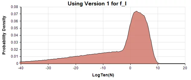
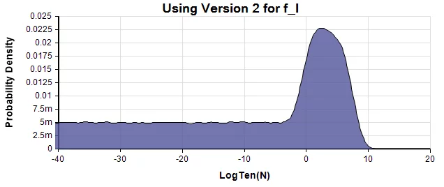
SDO reflect the lack of information on f_lfl by the immense range of uncertainty for in both versions of their model. Here is their probability density function (PDF) for f_lfl:
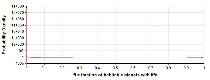
The PDF looks similar for Version 1 and Version 2, with spikes at f_l\approx 0fl≈0 and f_l\approx 1fl≈1, and little probability mass between these extremes. In Version 1 the spikes are roughly equal, whereas in Version 2 the spikes at f_l\approx 0fl≈0 and f_l\approx 1fl≈1 have about 84% and 16% probability respectively. In other words, there is a 16% chance that almost every habitable planet develops life, and an 84% probability that essentially none do. (The Earth did, of course, but this isn’t inconsistent with f_l\approx 0fl≈0 since these values are positive, just extremely small.) Thus, the distribution nearly degenerates into a Bernoulli (point) probability distribution. A Bernoulli point probability f_l=0.16fl=0.16 would mean that 16% of habitable planets develop life, which is a somewhat different interpretation. To see this difference, we included f_l=0.16fl=0.16 in the results as a point of comparison (See the penultimate row of the table) above.
The core problem here is that the range they used for abiogenesis events per habitable planet, f_lfl, just seems implausibly large in both versions, with the 25-75 quartile ranging from 2e-15 to 4e+14. We think this may be too extreme. The nice thing about having a live model to play with is that it is possible to repeat the results using more sane alternatives.
Number of detectable civilizations
Because the model includes information about how uncertain each factor is, we can plot the probability distribution for NN, the number of detectable civilizations in the Milky Way. Here is SDO’s distribution as a PDF:
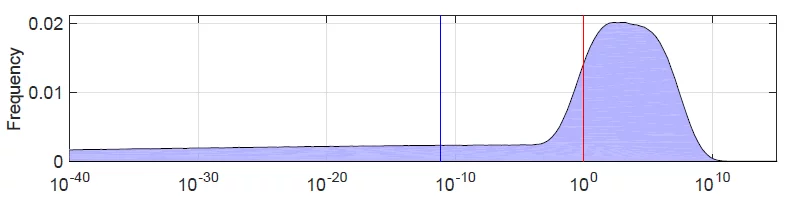
These two are from the Analytica model for the two versions for f_lfl.
The similarity between the first and third density, a combination of roughly LogNormal centered around Log(N)=2, and a LogUniform down to 10^{-160}10−160 suggests SDO used Version 2 of f_lfl for this graph. However, as we mentioned, the numbers given in the text are more consistent with Version 1.
A probability density at a particular x value is obtained by estimating (by Monte Carlo simulation) the probability that the true value is within a small interval of width \epsilonϵ around x, and then dividing by \epsilonϵ to get the density. The probability density of \log_{10} Nlog10N is not the same as the density of NN since the denominator is different. Although SDO label it the graph as the probability density of N, they are actually showing the density of \log_{10} Nlog10N, which is a sensible scale for order-of-magnitude of uncertainty. They label the vertical axis as “frequency” rather than probability density, likely an artifact of the binning algorithm used to estimate the densities.
Cumulative Probability Functions (CDFs) avoid these complications — the y-scale is cumulative probability, whether you plot NN or \log_{10} Nlog10N:
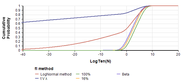
These CDFs show a dramatic difference between Version 1 (using the LogNormal method) and Version 2 (using the t V \lambdatVλ method), and between those versions and ours that remove the massive lower tails. An interesting aspect of these graphs are their qualitative shape. In the PDF, they all have the familiar bell-shaped body, but the extreme left tail stands out as unusual. The previous section points out that both versions of f_lfl are so extreme the effective distribution is degenerate. We think this is a flaw. Hence, it is interesting to see how the graph changes when we set f_lfl to a less degenerate distribution.
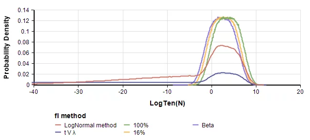
The LogNormal method for f_lfl, and the t V \lambdatVλ method are their Versions 1 and 2. The other three methods are less extreme. 100% and 16% use these as point probabilities for f_lfl, and Beta uses a Beta(1,10) distribution for f_lfl. The key conclusion of the paper that there is a significant probability that N is zero remains robust with these less extreme distributions for f_lfl.
Bayesian updating on Fermi’s observation
Fermi’s question “where is everybody” refers to the observation that we haven’t detected any extraterrestrial civilizations. SDO apply Bayes’ rule to update the estimates with this observation. To apply Bayes’ rule, you need the likelihoods P(¬D|N)P(¬D∣N) for each possible value of N, where ¬D is the observation that no ETI has been detected. SDO explore four models for this updating.
- Random sampling assumes that we have sampled K stars, none of which harbor a detectable civilization.
- Spatial Poisson assumes that there is no detectable civilization within a distance d of Earth.
- Settlement attempts to incorporate the possibility that interstellar propagation would be likely among advanced civilizations. It introduces several new parameters, including settlement timescales and a geometric factor. It is conditioned on the observation that no spacetime volume near the Earth has been permanently settled.
- No K3 observed conditions on the observation that no Kardashev type 3 civilizations exist— civilizations that harness energy at the galactic scale. It presumes that if such a civilization exists, either in the Milky Way or even in another visible galaxy, we would have noticed it. Among other parameters, it includes one for the probability that a K3 civilization is theoretically possible.
We implemented all these update models in the Analytica model. Our match to the paper’s quantitative results is only approximate. We are not sure why the results are not precisely reproducible. It was quite challenging figuring out what parameters they used for each case, since the paper and its Supplement 2 left out many details. With the exception of the settlement update model, we were able to get fairly close at least in qualitative terms. We explored that space of possible parameter values for the Settlement model but were unable to match the qualitative shape of the posterior reported in the paper. The likelihood equation for the K3 update appears to be in error in the paper since it doesn’t depend at all on N, but a more plausible version that does depend on N appears in Supplement 2.
In our Analytica model, you can select which update model(s) you want to view, and graph them side-by-side, along with (or without) the prior. For example,
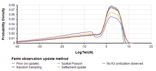
Once of the more interesting posterior results is P(N<1)P(N<1).
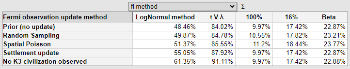
SDO report these numbers in Table 2 (in the same order as the rows of the above table) for P(N<1): 52%, 53%, 57%, 66%, 99.6%. We think they may have based their first 4 posteriors on Version 1. We are not sure about the K3 posterior, which differs substantially from our results.
In this table, we see that the models with a non-extreme, non-degenerate version of f_lfl are not substantially changed by the posterior update on the negative Fermi observation. These are the models that use a point estimate for f_lfl of 100% and 16%, as well as the one that uses f_l \sim Beta(1,10)fl∼Beta(1,10).
How to compute the posteriors
We explored two ways to implement these posterior calculations in Analytica. We found their results to be consistent, so we stuck with the more interesting and flexible method. This is interesting in its own right, and very simple to code in Analytica. The calculation uses sample weighting, in which each Monte Carlo sample is weighted by P(¬D|N)P(¬D∣N). The value for N is computed at each Monte Carlo sample, so from that P(¬D|N)P(¬D∣N) is also computed for each selected posterior method. The variable that computes P(¬D|N)P(¬D∣N) has the identifier P_obs_given_N. To compute the posteriors, all we had to do was set the system variable SampleWeighting to P_obs_given_N.
We also tried a second method for computing the posterior. It gives the same results, but is less elegant and more complex. This method extracts the histogram PDF(LogTen_N). It computes P(¬D|N)P(¬D∣N) based on the value of N that appears in the PDF. The product of the PDF column for LogTen_N and is P(¬D|N)P(¬D∣N) is the unnormalized PDF for P(N|¬D)P(N∣¬D).
We would expect this second method to perform better than the first method when the likelihood P(¬D|N)P(¬D∣N) is extremely leptokurtic. In this model, this is not the case.
Updating on a positive observation
The Fermi observation is the negative observation that we have never detected another extraterrestrial civilization. We thought it would be interesting here to explore what happens when you condition on a positive observation.
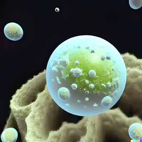
Extraterrestrial microbes
.jpg)
In March 2011, one of us (Lonnie Chrisman) attended a talk at Foothill College by NASA planetary scientist Dr. Chris McKay. Six years earlier, with the Huygens probe descending into the atmosphere of Saturn’s moon Titan, he and graduate student, Heather Smith, undertook a thought experiment. They asked: If there is life on Titan, what chemical signatures might we see? Especially, signatures that could not result from a known inanimate process? What would organisms eat? What would their waste products be?
At -190°C (-290°F), life on Titan would be very different, not based on water, but rather on liquid methane. Without knowing what such life forms would look like, they could still make some inferences about what chemical bonds organisms would likely utilize for metabolism. For example, the molecule with the most harvestable energy on Titan is acetylene ( C_2H_2 + 3H_2 \rarr 2 CH_4, \nabla G=80 kcal/moleC2H2+3H2→2CH4,∇G=80kcal/mole ). They published a set of proposed signatures for life in
C.P. McKay and H.D.Smith (2005), “Possibilities for methanogenic life in liquid methane on the surface of Titan“, ICARUS 178(1):274-276, doi.org/10.1016/j.icarus.2005.05.018
and then moved on to other work. Five years later, analysis of data from the Huygen’s probe and Cassini mission to Saturn found some unexplained chemical signatures.
Darrell F.Strobel (2010), “Molecular hydrogen in Titan’s atmosphere: Implications of the measured tropospheric and thermospheric mole fractions“, ICARUS 208(2):878-886, doi.org/10.1016/j.icarus.2010.03.003

These signatures matched those predicted as possible signatures of life by McKay and Smith 5 years earlier. One signature, a net downward flux of hydrogen, is particularly intriguing, since it implies that something is absorbing or converting hydrogen near the surface, for which no inorganic processes are known. The data remain ambiguous. For example, the Huygens probe did not detect a depletion of hydrogen near the surface, which is what would be expected if organisms on the surface are consuming hydrogen.
The interesting question here is how we should update our uncertainty based on a hypothetical future discovery of microbial life on an extraterrestrial body such as Titan. Such a discovery would influence our belief about n_ene, the number of planetary objects per star that are potentially habitable, as well as f_lfl, the fraction of habitable planetary objects where life actually starts. In our own solar system, it would make Jupiter’s moons Europa and Enceladus more likely candidates. Adding moons to planets as possible sites for abiogenesis would increase our estimate for n_ene by something like a factor of 3:
P( n_e | D ) =P(ne∣D)= LogUniform( 0.3, 3 )
To update f_lfl, we’ll use P( D | f_l, habitable) = f_lP(D∣fl,habitable)=fl, where D is the observation that this one additional planetary object is habitable and where life has emerged.
With these updates, the probability that there is no other intelligent contactable civilization would drop from 48.5% to 6.6%, and the probability that the galaxy is teeming with intelligent life would increase from under 2% to over 6%, using the Version 1 prior. Here is the table for different version of the prior (where only f_lfl varies between the 5 priors).
| P(N<1) — “we are alone” | P(N>100) — galaxy teeming with life | |||
|---|---|---|---|---|
| Prior | Posterior | Prior | Posterior | |
| Version 1 | 48.5% | 6.6% | 1.9% | 6.2% |
| Version 2 | 84% | 6.6% | 0.6% | 6.2% |
| f_l=100%fl=100 | 10% | 6.5% | 3.7% | 6.3% |
| f_l=16%fl=16 | 17% | 12.7% | 1.2% | 2.5% |
f_l \simfl∼Beta(1,10) |
23% | 13.6% | 1.4% | 2.4% |
It is interesting when comparing these priors how the extreme priors (Version 1 and Version 2) adjust to be nearly identical to the result obtained when setting f_l=100%fl=100. The f_l=100%fl=100 models the most extreme assumption that life always starts on every habitable planet. This reinforces our earlier criticism that the paper’s two versions of f_lfl are flawed. Because they are so extreme, they are roughly equivalent to saying life starts on a habitable planetary body either almost always or almost never. Thus the evidence that it happened on Titan would leave us with only the former option, that it happens almost always.
Summary
It is easy to be misled without realizing it when you estimate a single number (a point estimate) for an unknown quantity. Fermi’s question of why we never detected or encountered other extraterrestrial civilizations has spawned decades of conjecture for underlying reasons, yet Sandberg, Drexler and Ord show that there may be no paradox after all. We’ve reviewed and reimplemented the model they proposed. The possibility that there are no other detectable intelligent civilizations in the Milky Way is consistent with our level of uncertainty. The apparent paradox was simply the result of the “Flaw of Averages”.
We hope you are able to learn something by playing with the model. Enjoy!