On Tuesday I had an interesting exchange with Jorge Muro Arbulú, a professor in Peru, about the Cauchy distribution, which also called the Lorenzian distribution. Unlike most probability distributions you encounter, the mean and variance for strange distribution do not exist! How is it then, Jorge asked, that Analytica is able to compute the mean and variance? As he asked the question, he demonstrated Analytica computing the mean and variance in an example model.
Not only is this an excellent question, but it also reminded me of how I encountered this distribution last year in a theorem by Martin Arjovsky and Léon Bottou that resolved a problem in a deep learning model that I had been debugging at the time. That’s pretty cool, because I find it unusual for such an oddity of a distribution to be relevant to a real problem, let alone one that I’m working on! The Cauchy distribution arises in resonance and spectroscopy applications in physics, but in my case it came to the rescue in a deep learning project.
Read on and I’ll introduce you to this strange distribution, address Jorge’s question, and tell you about how it ended up relevant to machine learning.
The Cauchy Distribution
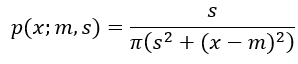
The cumulative probability function for the Cauchy is given by
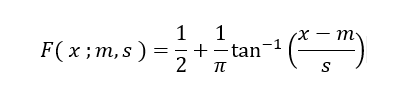

The parameters of the distribution are m, the mode, and s, the scale. The Cauchy distribution describes the position of x in the following triangle when the angle a is uniformly distributed between –![]() /2 and
/2 and ![]() /2.
/2.

From trigometry, you’ll remember that for this triangle, ![]() . Let ax be the angle corresponding to a particular x, then
. Let ax be the angle corresponding to a particular x, then

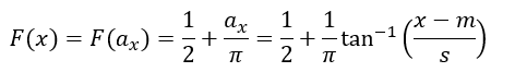
which gives us the cumulative probability function. The second equality above expresses the uniform distribution on a, and the third equality substitutes the trigometry relationship. The density is obtained by taking the derivative of F(x;m,s).

It is easy to generate Monte Carlo samples from a Cauchy. Just select the angle a from a Uniform(90,90) — in degrees here, and solve for x — since Analytica’s tan wants the angle in degrees, use m+s*Tan(Uniform(90,90)).
Mean and Variance undefined??
[Pillai & Meng, 2015] write
The Cauchy distribution is usually presented as a mathematical curiosity, an exception to the Law of Large Numbers, or even as an “Evil” distribution in some introductory courses.
Many of us may recall the surprise or even a mild shock we experienced the first time we encountered the Cauchy distribution. What does it mean that it does not have a mean?
I find the non-existance of the mean to be mindblowing. It isn’t a case where the mean is unbounded, it is that it really doesn’t exist, more akin to zero divided by zero. When I first wrote down the integral for the expected value as
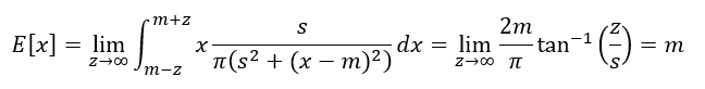

out popped a mean. So why do they say the mean doesn’t exist? Eventually, I had to ask my daughter to resolve this one for me. Take the same approach, but change the integration bounds:
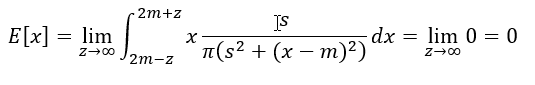

In both cases, were taking a limit to the same -∞ to ∞ bounds, but getting two different answers. And because of that, we say the mean doesn’t exist. In fact, for different choices of integration bounds, out pop different limits. The mean isn’t uniquely defined, you can essentially make it anything you want. I find it hard to wrap my head around that one.
The variance diverges in a more obvious way, where it makes sense to talk about it having infinite variance.


To use the Cauchy aka Lorenzian distribution in Analytica, add the Distribution Variations library to your model, and then use the function Lorenzian(m,s).
Here is a Lorenzian(5,2) plotted from 1000 latin hypecube samples:
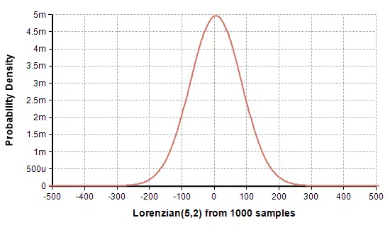
From the statistics view, you can read off a mean of 5.00 and standard deviation of 63.25. So if the mean and variance don’t exist, how is it that Analytica was able to compute them?
To understand the paradox, I ran a simple experiment. I generated 10 million independent random samples from the Lorenzian(5,2) distribution (monte carlo), and at each step, at each sample I computed the variance of the samples so far. Here is the running variance over the first 4M samples:

When you run an experiment like this on a better behaved distribution, what you’ll usually see is the variance converging to its true value as sample size grows. Here though, there is a trend towards larger and larger variances as the experiment proceeds. Basically, the vast majority of the samples are between -10 and 10, but every now and then it gets a whopping outlier, so big that it pushes the variance up. Then as it goes for a while without another whopping outlier, additional small samples cause the variance to decrease until wham!, another big outliner drives it up even further. Near the 3.75Mth sample, it got one that was so big (actually big negative), it pushed the variance up so much it became hard to see the interesting detail in the <4M range:
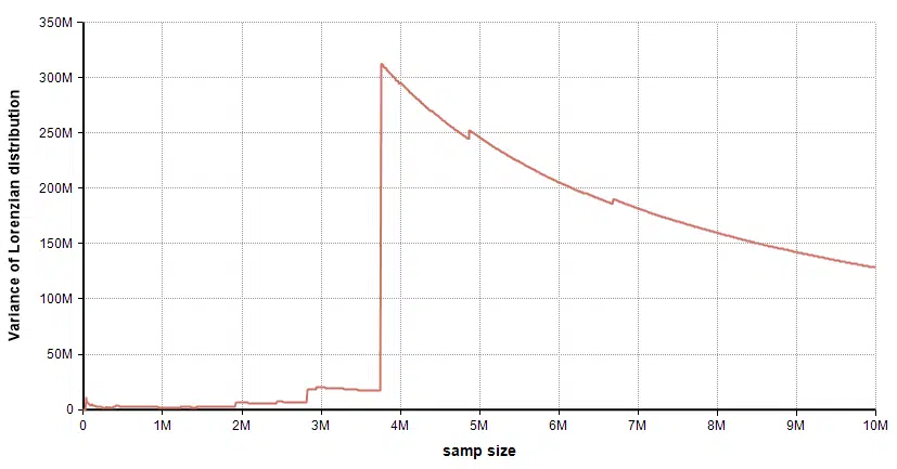
If you were to continue with this experiment to infinity, you could set any positive limit on the Y-axis — even at 10^100, and if run long enough, the variance will eventually plow through that limit!
Here is the running mean during this experiment:
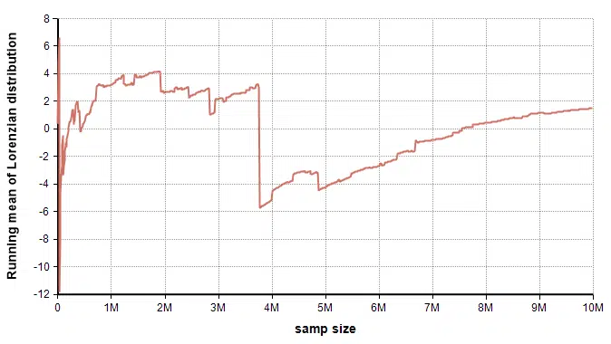
With the mean, these wild outliers clearly cause large jumps, but there isn’t any clear net growth effect. It is hard to say whether it is converging to something. So found the mean of 1 billion samples and repeated that experiment 50 separate times.
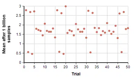
No single convergence value stands out, but it does seem interesting that the sample mean landed between 0 and 3 in all 50 trials.
Anyway, coming back to Jorge’s original question — how is it that Analytica can compute the mean and variance if these don’t exist? We’ve seen that it is easy to sample from a Cauchy distribution, and that you can always compute the sample mean and the sample variance for any sample. This is what Analytica was doing. But neither sample mean nor sample variance is meaningful in the case of Cauchy, and if you were to repeat the experiment, or up the sample size, it would not compute same same estimates consistently.
Relevance to machine learning
My wife will attest that my obsession with Generative Adversarial Networks (GANs) began last fall, since she had to put up with me talking about it constantly. The GAN is a deep learning architecture introduced by [Goodfellow et al., 2014] which learns to generate random samples from highly complex huge-dimensional complex probability distributions. Papers showing applications of GANs are being published at a phenomenal rate (see The GAN zoo).
In a GAN, two deep learning networks are trained: G(z) and D(x). The first network, G(z), is called the generator and accepts a random vector z as input, and outputs a “sample” point, x∈Rⁿ, where n is usually very large, and where the n dimensions have a highly complex correlational structure. In other words, G(z) learns to map from a random vector z to a representative sample from the target distribution P(x) that training instances are drawn from. The second network, D(x), is called the discriminater, and its job is to detect whether x was sampled from the “real world” (actually sampled from P(x)), or is a fake generated by G(z). During training, G’s objective is to fool D, whereas D’s objective is to learn not to be fooled. The training process is thus an adversarial “game” between D and G.
Training a GAN is notoriously difficult. In my own attempts, I witnessed good progress near the beginning of training. G started producing samples that looked fairly convincing and had pretty good coverage of the full sample space. But as training continued, G would fixate on the cases it was best at and suddenly stop producing samples other cases that it was less skilled at. For example, when simulating hypothetical loads on the electrical grid, initially it would generate data that resembled sunny days, data that resembled run-of-the-mill days, and samples that resembled windy days. But as training progressed, it seemed to figure out that it was really good at simulating the typical winter day and after a while that’s all it generated. Extremely few or no sunny days, run-of-the-mill summer days, windy days, etc. In the GAN field, this is called “mode dropping”. But really there are two phenomena here — one is the eventual absence of some “modes”, the other is the divergence from a reasonable representative “concept” to one that is less representative. The divergence issue was to me the most puzzling, because the objective function(s) promote the generation of samples that more closely match the true distribution. Given that the objective function points in that direction, why would it diverge? That was the mystery, and my key barrier to successful training. This became an impetus for me to do lots of theorizing, experimentation, reading and analysis (this was my obsession at the time, after all). The Cauchy distribution made its appearance with the first experimentally-consistent explanation for this behavior that I found, appearing in Theorem 2.6 of [Arjovsky and Bottou, 2017].
Training on MNIST
The MNIST dataset contains 60,000 black & white images of hand-written digits, 28×28 pixels in size. The goal is to train a network, G, that can generate random images that are indistinguishable from actual hand-written digits. Furthermore, since MNIST contains the same proportion of each of the 10 digits (0 thru 9), the learned network ought to generate images of “3” with the same frequence as images of “1”s. GANs don’t just memorize the training data, they learn to generate representative samples that they’ve never seen before, but which appear to come from the target distribution. Notice here that the sample space is R784, i.e., 784 dimensions.
I conducted a variety of experiments using two 3-layer Linear-ReLu nets, D and G. In the base case, D was alternatively exposed to a true training image and then to a G(z) for a uniform random z vector using the currently trained generator up to that time, and then G was updated by backpropagating through the generator. This was standard stuff direct from the original paper
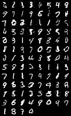
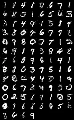
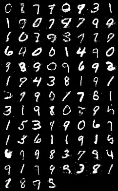
They are starting to become recognizable, and there appears to be a fairly reasonable sampling of nearly every digit. By 200 epochs, it has refined them even further:

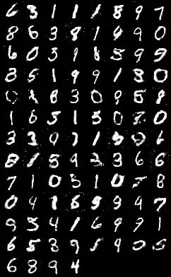
but then things went downhill from there. As it progressed, it showed a propensity for “1”s, “7”s and “9”s, and I saw the other digits appear less and less frequently, until by the 1000th epoch, it was completely fixated on its favorites.

To aid with experimentation, I wanted a way to automatically measure the coverage of the different digits as training progressed and as I compared variations on network architectures, algorithms, and parameters. For that, I independently trained a Convolutional Neural Network (CNN) on the MNIST dataset, and used it to classify G’s output into one of the 10 digits. To measure the amount of coverage, as training progressed, I periodically had G generate 100 random images, classified them into digits, computed the entropy and graphed it.
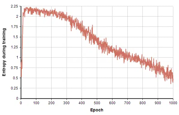
Perfectly uniform coverage of all 10 digits would have an entropy of Ln(10) = 2.3. The graph makes the good initial coverage followed by the gradual decline with more training apparent.
At the time, [Arjovsky & Bottou, 2017] hadn’t been published yet, but there were a lot of other people exploring this same thing and a lot being written. One point of broad consensus at the time seemed to be that these phenomena occurred when G trained faster than D (we now know that if anything, this wisdom was backward). So I conducted experiments to test these theories in various combinations. For example, for every 1 epoch of G, train D for 2 epochs (blue) or train D for 5 epochs (green):
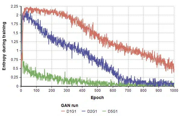
Not only did this collapse faster, they collapsed more thoroughly to the point where they only generated “1”s. I conducted numerous other experiments to test many other hypotheses and alleged wisdom by others in the field, but they all experienced this mode collapsing divergence, until…
The Cauchy distribution makes its appearance
The paper by [Arjovsky & Bottou, 2017] is one of the best papers that I’ve seen in the GAN field. Their primary theorems elucidated why mode collapse occurs in the most convincing manner (to me) up to that point. The same authors had developed these theoretical underpinnings in earlier papers (esp. [Arjovsky, Chintala and Bottou, 2017]) where they introduced the Wasserstein GAN. The core theoretical idea is that the output sample space accessible to G is a substantially lower-dimensional manifold embedded in the higher-dimensional output space. For example, the manifold’s dimensionality can’t exceed the size of the vector z, which is much smaller, here 100 compared to 784 dimensions in the MNIST output space. The manifold creates “gaps” which the objective metric, which for standard GANs implied a Jensen-Shannon divergence measure, can’t “see” across. Hence, it gets stuck on a manifold and can’t “see” the gradient signal from the next “fold” over, where perhaps a different mode resides. Their main result, which had a tremendous impact on the field, was that the crux of the problem was in the objective function. Other divergence measures (notably, they argued, the Wasserstein divergence) are less susceptible to these problems. This isn’t the end of the story, because there are some issues with the implementation of the Wasserstein divergence metric, but that’s not today’s topic. For me, however, the real gem in the paper was a secondary theorem, buried down later in the paper — their Theorem 2.6….
The original paper that introduced the GAN, [Goodfellow et al, 2014], proposed using the following objective function for training

The min-max reflects the 2-player game ensueing between G & D, and it is well-known that this objective implies a minimization of the Jansen-Shannon divergence between the target and learned distributions. However, that same paper went on to explain how the log(1-D(G(z)) term is flat at the beginning of training, leading to very little gradient signal and poor training, especially near the beginning of training. So, they proposed replacing Log(1-D(G(z))) with -Log(D(G(z)) and claimed it made all the difference in the world. The new objective appears to provide the training with similar incentives, and is also maximized when the generator’s distribution is equal to the true distribution. They were quite convincing, and as a result I believe that almost everyone training GANs, including myself, were using the modified objective. Although there had been many (probably dozens) of papers that have analyzed the JS objective in numerous ways, [Arjovsky & Bottou, 2017] were the first to analyze the modifed objective. They found that the modified objective corresponds to a divergence metric equal to KL(Q|P) – 2JS(Q|P), where Q is G’s distribution — basically it is a difference of a Kullback-Liebler divergence and a Jensen-Shannon divergence. The negative on the JS is pushing the learned distribution away from the target distribution, so there is a fight ensuring between KL and JS. The KL is non-symmetric in its distribution paramaters, and in this case is reversed from the usual KL divergence used in maximum likelihood learning. This has the effect of amplifying the penalty for fake-looking samples and reducing the penalty for mode dropping. Because the JS is symmetric, it doesn’t alter that trade-off. And all this combines to create an unstable gradient that is characterized by a Cauchy distribution.
The specific theorem says that when you consider random tweaks to the weights in the discriminater network, D, then those minor permutations cause the expected gradient
![]()
to change in a manner characterized by a Cauchy distribution. In this equation, z is sampled randomly (from me p(z) was a uniform-random vector, some people use gaussian random vectors), and for a given G and D, the result is a deterministic vector (across all weights, theta). The theorem considers the sensitivity of this expected gradient to minor changes in the weights of D, i.e., “noise”. They model that noise as 0-mean Gaussian. As you make these small moves, the gradient changes as well, and these changes to the gradient were independently modeled as a gradient. From that, their Theorem 2.6 shows that the expected gradient (in the preceding equation) follows a Cauchy distribution. The result follows quite directly from these assumptions — the gradient chain rule applied to the a log(D(…)) function puts a partial derivatives of D in the denominator and D( ) in the numerator, where these Gaussian assumptions yield a normally-distributed term in the numerator and a zero-centered normally-distributed term in the denominator. The ratio of normally distributed random variables has a Cauchy distribution.
Now that you know about Cauchy distribution, consider what that means. During learning, the training tweaks the weights this way and that. They tweak in all sorts of directions, and although it isn’t entirely random, this idea of modeling these tweaks with a Gaussian distribution seems like a reasonable way of characterizing those dynamics. Most of the gradients will come out pretty well behaved, but then those outlier gradient occur, causing it to jump out of whatever stablity it might have found. This makes it intrinsically unstable.
Testing the Cauchy hypothesis
The Cauchy result from Theorem 2.5 and 2.6 of [Arjovky & Button, 2017] sent a strong signal that you shouldn’t use the -log(D(G(z)) alternative from [Goodfellow et al, 2014]. To that point, I had not actually explored the impact of that approximation. In my final MNIST experiment reported here, I returned to the original base-case model, but replaced the -Log(D(G(z)) objective term with the vanilla Log(1-D(G(z))) objective — i.e., a straight Jenson-Shannon divergence metric. I cal this “D1G1 pure”, since D and G are each updated once per epoch and the objective is the pure one. The result is the red line.
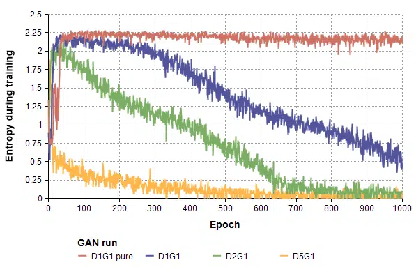
Notice that the “pure” Jensen-Shannon divergence metric shows no divergence in coverage. As predicted by [Goodfellow et al, 2014], it did start out a bit slower, but that was far offset by the stability. The next two images show generated samples after 100, 500, and 1000 epochs respectively.
In short, their Cauchy theorem seems to have pinpointed the underlying cause for the divergence in my own experiments.
Summary
The Cauchy distribution, also called a Lorenzian distribution, is a strange creature. It’s primary application seems to be for teaching students of probability that some distributions don’t have a well-defined mean and variance.
The original question was: How is it that Analytica can compute the mean and variance when these don’t actually exist? The resolution to this paradox is that it is easy to generate samples from a Cauchy, and you can always compute the sample mean and sample variance. But as you increase sample sizes, these don’t stabilize.
This distribution is strange, which is why I found it so interesting when I saw it appear last year in the context of training Generative Adversarial Networks, in what actually turned out to be a very useful result for a pragmatic problem I was working on.
References
- Martin Arjovsky and Léon Bottou (2017), “Towards principled methods for training Geneative Adversarial Networks“, Fifth International Conference on Learning Representations (ICLR), arXiv preprint arXiv:1701.04862.
- Natesh S. Pillai and Xiao-li Meng (2015), “An unexpected encounter with Cauchy and Lévy“, (PDF), The Annals of Statistics 44(5): 2089–2097.
- Ian J. Goodfellow, Jean Pouget-Abadie, Mehdi Mirza, Bing Xu, David Warde-Farley, Sherjil Ozair, Aaron Courville, and Yoshua Bengio (2014). Generative adversarial nets. In Advances in Neural Information Processing Systems 27, pp. 2672–2680.
- Martin Arjovsky, Soumith Chintala, Léon Bottou (2017), “Wasserstein GAN“, preprint arXiv:1701.07875.
- The GAN Zoo: A list of all named GANs
- The online integral calculator
- “Cauchy distribution” at Wolfram Mathword.
- Lorenzian() distribution function on the Analytica Wiki
- Yann LeCun, Corinna Cortes, Christopher J.C. Burges, “The MNIST database”.