The infection fatality rate (IFR) of COVID-19 is one of the most important parameters for mathematical models of the pandemic, yet it remains largely a mystery because we don’t yet know how many people have actually been infected. The IFR is the number of people who die from COVID-19 divided by the number of people who get infected. When you see the number of reported cases each day in the news, these reported cases include only people who have been diagnosed as having COVID-19 disease, or who have tested positive, but it does not include people who never get tested or are asymptomatic. Therefore, studies to assess the total number of infections are super important. This morning the results of a large-scale Stanford University study that tested for the presence of antibodies in the population of Santa Clara County, California were released.
When conducting a large-scale community antibody test like this, the most important aspect of the experimental design is to make sure that the people selected for testing don’t self-select for the study. People who have reason to believe that they may have had COVID-19, or may have been exposed, will be vastly more eager to get tested than people who have no reason to think they may have had it. Ideally, you would either test everyone, or you should randomly select the participants without simply asking people to participate. If people self-select, this self-selection bias will result in a population of test subjects who are far more likely to have had the disease than the general population.
Today’s study is a very important one, and the researchers did a lot of other things right, but unfortunately they let participants self-select, so I believe that their reported results have overestimated the true prevalence in Santa Clara County. In this posting, I examine how to adjust their results to account for the self-selection bias.
How participants were selected
The following description of how participants were recruited is taken directly from their paper:
We recruited participants by placing targeted advertisements on Facebook aimed at residents of Santa Clara County. We used Facebook to quickly reach a large number of county residents and because it allows for granular targeting by zip code and sociodemographic characteristics. We used a combination of two targeting strategies: ads aimed at a representative population of the county by zip code, and specially targeted ads to balance our sample for under-represented zip codes. In addition, we capped registration from overrepresented areas. Individuals who clicked on the advertisement were directed to a survey hosted by the Stanford REDcap platform, which provided information about the study.
Basically, they put out a targeted ad on Facebook. Although it doesn’t say so here in the paper, I have heard second hand from people here in Santa Clara county that the ad offered a 10 Amazon gift card to participate. They targeted the ad to a subset of the population in each zip code.
They made substantial efforts to obtain a representative sample from the different zip codes and demographic groups within the county, and then after the proportions of participants didn’t quite match these distributions, they adjusted their results for this aspect of sampling bias. Their attention to this aspect of sampling bias was good. But they made no adjustments for self-selection bias.
All subjects’ blood were drawn for testing on 3-Apr-2020 or 4-Apr-2020 in three drive-through test sites in Los Gatos, San Jose and Mountain View.
The study’s results
After eliminating some subjects for various technical reasons, the study ended up with 3,300 people with test results. Of those, 50 were positive test results, constituting 1.50% of the tests. After adjusting for demographic and geographic sampling biases, they adjusted this to an estimate of 2.81% positive. They then adjusted for the accuracy of the test (the actual accuracy is uncertain) to come up with a final estimate of prevalence between 2.49% to 4.16% percent, where the range is due to assumptions about the test’s accuracy. This prevalence translates to between 48,000 and 81,000 people in the county, which is 50-85 times the number of confirmed cases. This led to an IFR of 0.12% to 0.2%.
The results I just listed are directly from the paper. None of these results are adjusted for self-selection bias.
Self-selection adjustment
Suppose that people who have previously had COVID-19 are 10 times more likely to sign up for a test than people who have never been infected. This is called the likelihood ratio, which I’ll denote as L. In this example, L=10.
Let C denote whether a person has had COVID: C=true if they have, C=false if they haven’t. Let T denote whether that person enrolls in the test: T=true means they enroll, T=false means they don’t. With this notation, Bayes’ rule can be written as
[ odds( C | T ) = odds( C ) cdot L ]Where odds(C|T) is the odds a person had COVID-19 given that they take the test, and odds(C) is the odds a person from the general population had COVID-19. The study determined odds(C | T), whereas what we care about is odds(C), which doesn’t have the self-selection sampling bias.
The study estimated the prevalence, p, which is related to odds as odds(C|T) = p / (1-p). With some simple algebra, the true prevalence is obtained by multiplying the study’s estimate by an adjustment, alpha, given by
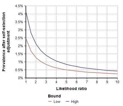
[ alpha = {1 over { L (1-p) + p }} ]This adjustment is shown in the following graph as a function of the likelihood ratio.

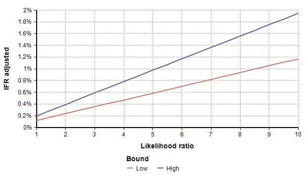
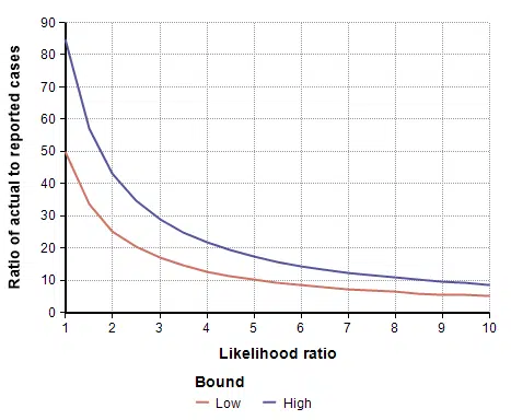
To adjust for self-selection bias, you need to estimate how many times more likely a person who had previously had COVID-19 would be to participate in the study, compared to a person who has never had it. This is the likelihood ratio. If you think that person would be 2.5 times as likely, use the self-selection adjustment for L=2.5 from the above graph, which is alpha=0.4, and then multiply the study’s prevalence number by 0.4, which yields a prevalence between 1.00% and 1.69%. You can also multiply by alpha to adjust the total number of infected people, which for L=2.5 is between 19,500 and 33,000. To adjust the IFR estimate, divide by alpha, which yields an adjusted IFR estimate between 0.29% and 0.49%. Adjusted values for these results are shown in the next four graphs as a function of likelihood ratio, the two lines showing the lower and upper estimates.

Estimating the Likelihood ratio
To adjust the study’s results, you have to estimate the likelihood ratio — how many times more likely someone previously infected would be to participate compared to someone never infected. Of course, this is also a big unknown.
Because the person considering whether to register doesn’t know whether she has COVID-19 or not, you might find the likelihood ratio to be overly abstract. It is easier to compare how much more likely it would be for someone who had symptoms at some point to participate in the study than someone who never had any symptoms. Of course, you might also want to consider the possibility that a person may be more likely to register because they know they had come into contact with someone else, or because their job makes them more vulnerable, etc. Because there are these other possibilities, I chose not to decompose the likelihood ratio into other estimations.
I live in Santa Clara County, and I was aware that the study was taking place. Many of my family’s friends were also aware that it was taking place, and we know of at least one person who tried very hard (unsuccessfully) to find the ad so that she could participate, because as she said, she had been sick and wanted to know if she had had COVID-19. Hence, based on my own experiences, my personal guess is L=5. But there is nothing magic about my guess, yours may differ.
Summary
The results from today’s study may lead some people to conclude that COVID-19 is no worse than the common flu. But this adjustment for self-selection bias show that this is not true. As the graphs above show, the prevalence drops off quickly when adjusted for even a small self-selection bias.
Understanding how many people in the population have had COVID-19 is an extremely important parameter for mathematical models of the pandemic. It is a critical piece of knowledge for determining how deadly a COVID-19 infection really is, for projecting hospital capacity and how many people may die, and for deciding when the economy can be reopened. Large scale tests of the population, like the Stanford study published today, help us estimate the prevalence of COVID-19 in the population.
When conducting a large-scale prevalence study, it is important to eliminate self-selection bias. When people are allowed to decide whether to participate in the study, those who have reason to believe that they are more likely to have had it will be more likely to participate. This may include people who had suspicious symptoms at some point, who know they were exposed at some point, or who work in situations that put them at greater risk of infection. In this article, I discussed how we can attempt to adjust for self-selection bias in the large-scale Santa Clara County study that was published this morning.